Presenter - Dynamic Online Pricing Using MAB Experiments

00:01

Profiting Efficiently and Pricing Dynamically

Reinforcement learning + Economics

Start

Pricing: exploration-exploitation tradeoff

This paper provides an elegant solution to solve exploration-exploitation tradeoff in a "cold-start" pricing problem.

Exploration & Exploitation

need experimentation to learn demand curve before setting the optimal price (cold-start)
finding optimal price earlier ensures a higher profit

Solution: fine-tuned UCB algorithms

tuning exploration bonus item: considering price $p_k$ and uncertainty $2\hat{\delta}$
"shutoff" rule: do not explore dominated options

Contributions

a novel combination of economic theory with machine learning to solve pricing problem
introduce distribution-free theory of demand to improve existing algorithms theoretically and empirically

Short Summary

Model setup

Modified Algorithms

Some Thoughts

Pricing with Federated Learning

○○○○

current

Pricing: exploration-exploitation tradeoff

This paper provides an elegant solution to solve exploration-exploitation tradeoff in a "cold-start" pricing problem.

Exploration & Exploitation

need experimentation to learn demand curve before setting the optimal price (cold-start)
finding optimal price earlier ensures a higher profit

Solution: fine-tuned UCB algorithms

tuning exploration bonus item: considering price $p_k$ and uncertainty $2\hat{\delta}$
"shutoff" rule: do not explore dominated options

Contributions

a novel combination of economic theory with machine learning to solve pricing problem
introduce distribution-free theory of demand to improve existing algorithms theoretically and empirically

The last comment block of each slide will be treated as slide notes. It will be visible and editable in Presenter Mode along with the slide. Read more in the docs

Profiting Efficiently and Pricing Dynamically

Reinforcement learning + Economics

Start

Pricing: exploration-exploitation tradeoff

This paper provides an elegant solution to solve exploration-exploitation tradeoff in a "cold-start" pricing problem.

Exploration & Exploitation

need experimentation to learn demand curve before setting the optimal price (cold-start)
finding optimal price earlier ensures a higher profit

Solution: fine-tuned UCB algorithms

tuning exploration bonus item: considering price $p_k$ and uncertainty $2\hat{\delta}$
"shutoff" rule: do not explore dominated options

Contributions

a novel combination of economic theory with machine learning to solve pricing problem
introduce distribution-free theory of demand to improve existing algorithms theoretically and empirically

Model Setup: Demand

Utility function:

u_i = v_i − p

We assume heterogeneity among consumers can be separated as observable (by descriptive variables $Z_i$ ) and unobservable heterogeneity.

v_i = f(Z_i) + \nu_i.

Segments: the firm assign consumers into segments $S$ , and $s \in S$ represents combination of descriptive variables $Z_i$ .

$v_s$ : observable heterogeneity
$\nu_i$ : unobservable heterogeneity, also the "quality of segments"

v_i = v_s + \nu_i, \nu_i \in [-\delta, \delta]

Model Setup: Supply

A monopolist determines the price with information that the consumer valuation is $[v_L, v_H]$

No price discrimination: do not use segmentation information to change the price

Model Setup: MAB Pricing

Profits: The firm can determine the price from price set $p \in \{p_1, p_2, ... p_k\}$ and face with demand $D(p)$ , thus the profit is $\pi(p) = p D(p)$ .

Price experimentation: Suppose by time $t$ , the firm has charged $p_k$ a total of $n_{kt}$ times. Let $\pi_{k,1},\pi_{k,2},\ldots,\pi_{k,n_{kt}}$ be realizations of profit per consumer from every time that price $p_k$ has been charged.

We assume that these are drawn from an unknown probability distribution with a mean at the true profit $π(p_k)$ .

Pricing problem:

\begin{aligned}p_t=\Psi(\{p_\tau,\pi_\tau|\tau=1,\ldots,t-1\})\end{aligned}

Test

Criterion of performance

Use maxmin regret: minimizing the maximum deviation to optimal profit.

\begin{aligned} \mathrm{Regret}(\Psi,\{\pi(p_{\mathbb{k}})\},t)& =\mathbb{E}[\sum_{\tau=1}^{t}\pi^*-\pi_{p_\tau}] \\ &=\sum_{\tau=1}^t(\pi^*-\pi(p_\tau)) \\ &=\pi^*t-\sum_{k=1}^K\pi(p_k)\mathbb{E}[n_{kt}] \end{aligned}

UCB algorithm

UCB algorithm is the sum of "expected reward" and an "exploration bonus".

UCB1, Auer (2002)

\text{UCB}1_{kt}=\bar{\pi}_{kt}+\sqrt{\frac{2\log t}{n_{kt}}}

Assume the profits of different prices are uncorrelated

23
23232

Here the bonus term can be written as $\sqrt{\frac{\alpha\log t}{n_{kt}}}$ when $\alpha=2$ , and the paper proposed another value to achieve better performance.

Learning the Demand Curve from Price Experiments

Repeat-purchase data can help to backout consumer preference.

For example:

She purchases at $3
does not purchase at $8
purchases at $2
does not purchase at $6

then her preference lies between $3 and $6.

However, this case is overly restrictive, thus the paper focus on cross-sectional learning across consumers.

Learning Segment-Level Demand with Partial Identification

Given consumer’s response, their potential preference types are bounded.

Preference: $\theta_s \in \{\theta_1, \theta_2, ... \theta_K\}$ , where $\theta_k > p_k$ and $\theta_{k} < p_{k+1}$

Three cases:

$D(p_k)_{s,t}=0$ , all consumers reject at price $p_k$ , then consumers possible types are $\{\theta_1, ...\theta_{k-1}\}$
$D(p_k)_{s,t}=0$ , all consumers accept at price $p_k$ , then consumers possible types are $\{\theta_{k}, ... \theta_{K}\}$
$D(p_k)_{s,t} \in (0,1)$ , only part of consumers accept, then types are combination of case 1 and 2

Estimation of price range $p_{min}$ and $p_{max}$ :

$p_{s,t}^{max}\equiv\min\{p_{k}|D(p_{k})_{s,t}=0\}$ , the minimal price allowing all consumers to reject
$p_{s,t}^{min}\equiv\max\{p_{k}|D(p_{k})_{s,t}=1\}$ , the maximal price allowing all consumers to accept

Note: do not use information of 3

For a consumer with preference range $[\$2, \$4]$ (Seg A accept and Seg B reject for sure, and same group size), then the probability of accepting $p_k = 3$ is specified as $0.5 = 1*0.5 + 0*0.5$ . They did not use 20% accept ratio in for Seg A when price is $3.

Learning Segment-Level Demand with Partial Identification

Summary

For partial identified $H_t[\pi(p_k)]=[LB_t(\pi(p_k)),UB_t(\pi(p_k))]$ , where:

$LB_t(\pi(p_k))=p_k\sum_{s\in S}\psi_s\mathbf{1}(\hat{v}_{s,t}^{\min}\geq p_k)$
$UB_t(\pi(p_k))=p_k\sum_{s\in S}\psi_s\mathbf{1}(\hat{v}_{s,t}^{\max}\geq p_k)$

That means for a given price, the weighted average of probability that each segment can accept/reject the price for sure.

Classical UCB algorithms

UCB-PI-untuned

\begin{align} \text{UCB}1_{kt}&=\bar{\pi}_{kt}+\sqrt{\frac{2\log t}{n_{kt}}} \\ \text{UCB-tuned}_{kt}&=\bar{\pi}_{kt}+\sqrt{\frac{\log t}{n_{kt}}\mathrm{min}\left(\frac14,\mathrm{V}_{kt}\right)} \end{align}

Next step:

prove that regret of UCB-PI is lower than UCB1
define a tuned version of the UCB-PI algorithm analogous to Audibert et al. (2009)

UCB with Partial Identification (PI)

UCB-PI and UCB-PI-untuned

\begin{align} \text{UCB-PI-untuned}_{k t}&=\{\begin{array}{ll} \bar{\pi}_{k t}+p_{k} \sqrt{\frac{2 \log t}{n_{k t}}} & \text { if } U B_{t}(\pi(p_{k}))>\max _{l} L B_{t}(\pi(p_{l})), \\ 0 & \text { if } U B_{t}(\pi(p_{k})) \leq \max _{l} L B_{t}(\pi(p_{l})) . \end{array} \\ \text{UCB-PI-tuned}_{k t}&=\{\begin{aligned} \bar{\pi}_{k t}+ & 2 p_{k} \hat{\delta} \sqrt{\frac{\log t}{n_{k t}} \min (\frac{1}{4}, \mathrm{~V}_{k t})} & \text{ if } U B_{t}(\pi(p_{k}))>\max _{l} L B_{t}(\pi(p_{l})), \\ 0 \quad & \text{ if } U B_{t}(\pi(p_{k})) \leq \max _{l} L B_{t}(\pi(p_{l})) . \end{aligned} \end{align}

Improvements in UCB-PI-untuned:

assign an action a zero value if the upper bound of potential returns is lower than the highest lower bound across all actions. Economically, we do not explore dominated options (the optimal return is still lower than the other lower returns).
scale the exploration bonus by price $p_k$ since the original reward in UCB1 is $[0, 1]$ but now $[0, p_k]$ for dummy demand.

Improvements in UCB-PI-tuned: add an additional tuning factor $2\hat{\delta}$ : size of uncertainty ↑ exploration bonus↑

Why…

Questions I have while reading the paper:

Stability assumptions in model: preference, budget, and outside option
- stochastic preference: empirical distribution of choices violates the rational choice theory
- in this paper we can find simulated data from field experiment silghtly violate it.
No strategic competetiton and Price discrimination

Questions I found while reading related papers:

Difficult to scale efficiently with high-dimensional characteristics
- in Carl Mela et al. (2023), added collaborative filtering under a recommender system framework
Stronger UCB variants
- Y Abbasi-Yadkori et al. (2011) adopted martingale inequality to derive preciser bound (Hoeffding inequality in classical UCB)

Questions when I connected the paper with reality:

e-commerce giants have multi-server issues

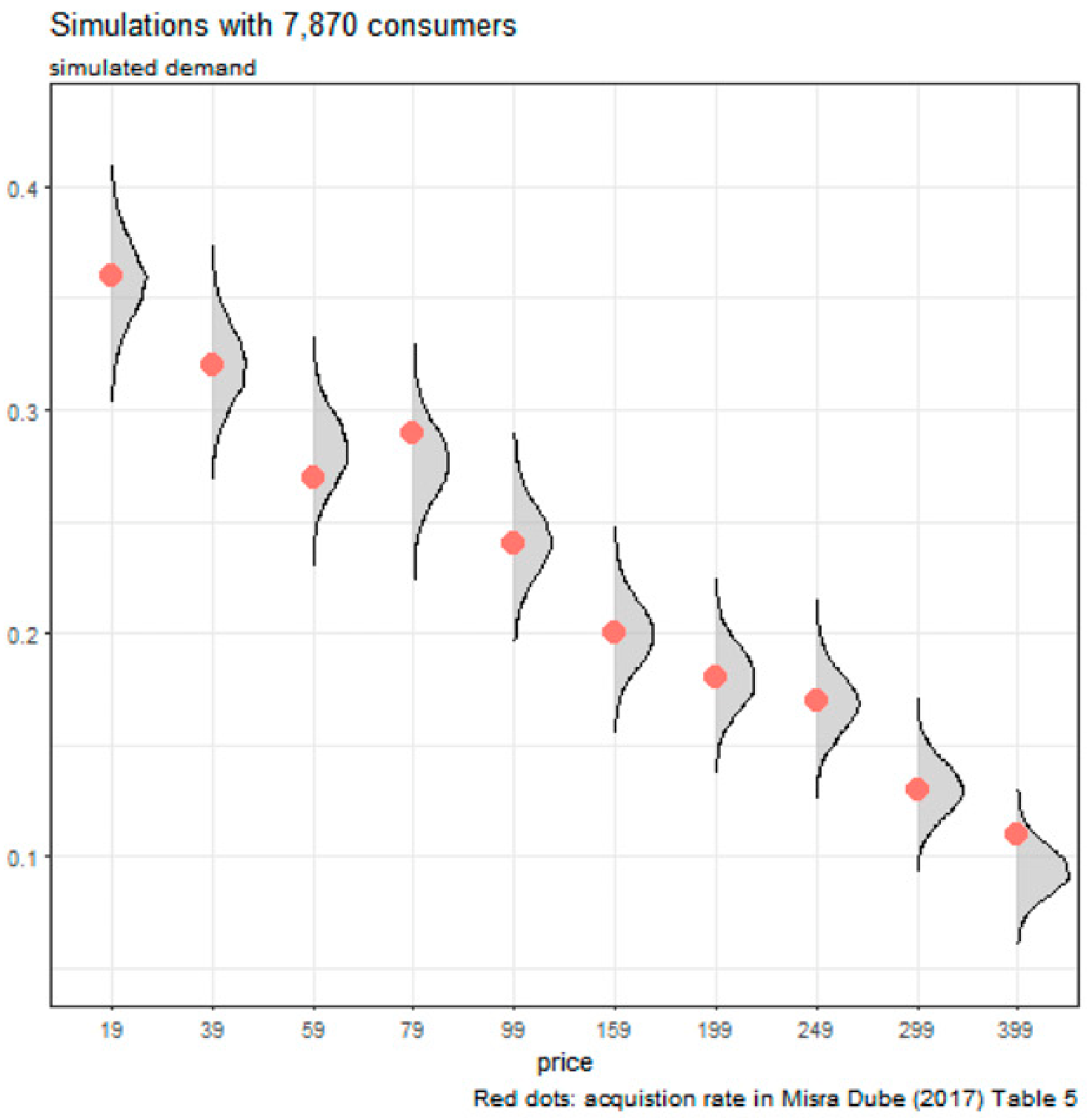
Simulated data in DM

When the price is 79, the demand shift upward.

Field Image — acquisition rate and price

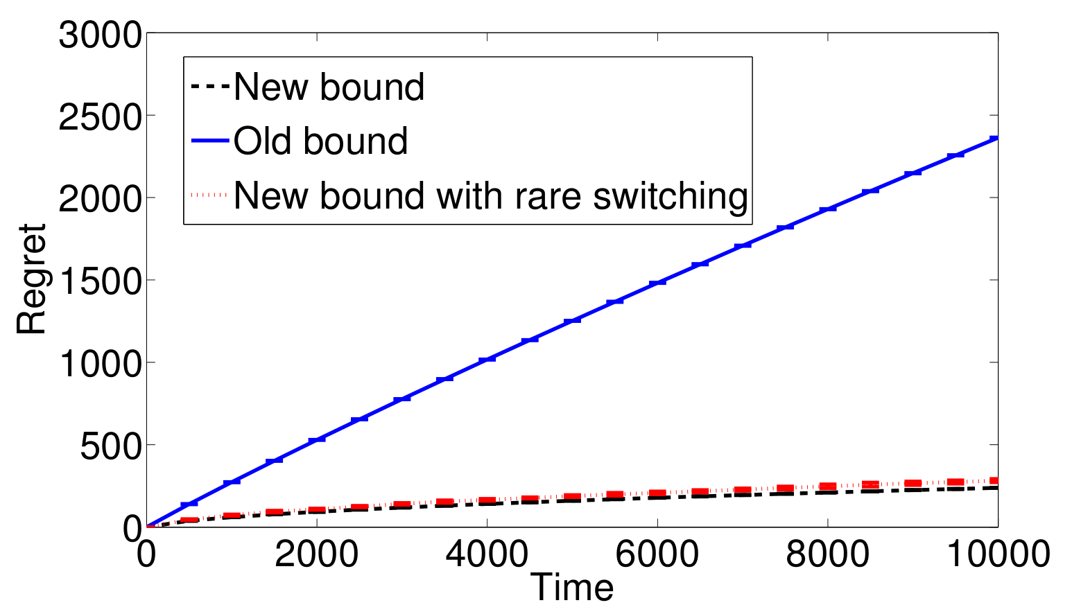
Better UCB

The modifed UCB has much better performance.

Pricing with Multi-servers

In this Big Data era, a "global optimal pricing strategy" is hard to find.

Lets say we wanna train a strategy for Amazon, we will find following problems:

Cannot access "whole data" since price experimentation data are stored in different servers
e.g. Amazon has data centers in many places like SFO (west) and IAD (east)
Local servers find a biased pricing strategy based on partial data, and a central server can communicate with local servers to find a global optimal strategy but incurs communication loss

Research Question: how to optimize the decentralized learning process using the same trick in Misra paper?

utlizing power of multi-servers and find optimal prices
improve the communication efficiency

Illustration

Problem Formulation

Utility, preference, price settings. follow Misra paper.

For the communication problem, I followed Shi and Shen (2021).

UCB with Federated Learning (Shi and Shen, 2021)

Non-iid data generation. Data in local servers $1, 2, ... l$ correlated with "whole data", but are non-iid. For segment $s$ , assume the true mean is $\mu_s$ , and the local mean follows $\mu_{s, l}$ where:

\mu_{s, i} \neq \mu_{s, j}, \quad i \neq j.

Communication Loss. Every time a central server communicate with local server to update the model and send back the model to each local server, it incurs constant cost $C$ .

Core difficulty

Shi and Shen (2021) developed Fed2-UCB algorithms to solve the Federated learning based on a stylized demand distritbution (normal distribution family), which might not apply to a distribution-free situation (Misra paper)

Misra paper mentioned that their proof differ from standard UCB proof

Intuition

we are considering this question: whether the optimal global pricing strategy is the combination of local optimal solutions?

with disitribution-free search in local servers, we may find suboptimal solution while updating the models